3-D Human pose estimation from monocular images or video is an extremely difficult problem. In this work, we present a hierarchical approach to efficiently estimate 3-D pose from single images. To achieve this, the body is represented as a graphical model and optimized stochastically. The use of a graphical representation allows message passing to ensure individual parts are not optimized using only local image information, but from information gathered across the entire model. In contrast to existing methods, the posterior distribution is represented parametrically. A different model is used to approximate the conditional distribution between each connected part. This permits measurements of the Entropy, which allows an adaptive sampling scheme to be employed that ensures that parts with the largest uncertainty are allocated a greater proportion of the available resources. At each iteration, the estimated pose is updated dependent on the Kullback Leibler (KL) divergence measured between the posterior and the set of samples used to approximate it. This is shown to improve performance and prevent over fitting when small numbers of particles are being used. A quantitative comparison is made using the HumanEva dataset that demonstrates the efficacy of the presented method.
Model Representation
The body is represented by a set of ten parts, each part has a fixed length and connected parts are forced to join at fixed locations. The conditional distribution between two connected parts, which describes the likely orientation of a part given that of the part to which it is connected, is modeled by first learning a joint distribution using a Gaussian Mixture Model (GMM). For efficiency all covariances used to represent limb conditionals are diagonal and can be partitioned. The state of each part represents a quaternion rotation that defines its orientation in the global frame of reference, which here is defined to be that of the torso. The location of a part is dependent on the state of the part to which it is attached.This is as parts are forced to be connected at fixed joint locations.
The benefit of learning a full conditional model between neighbouring parts is two fold. Firstly, consider an approach where two independent particle filters are used to locate the upper and lower arm respectively and suppose that each distribution has two modes. As the two particles filters are modeled independently how will the samples drawn from the second filter know to which mode in the first particle filter they are correlated with? Secondly, different GMM components learnt in quaternion space correspond to different spatial locations.
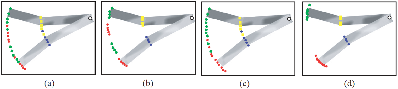 |
| Hypothetical two part example highlighting the difference in modeling different parts independently (a,b) and using conditional models (c,d). (a,c) show the prior model and (b,d) the model after a number of iterations. Both limb conditionals are represented by a two component mixture model where each component is represented by different colors. Whilst the conditional model can represent each observational mode by a single mixture component (d), the independent (unconditional) model can not and as such 'phantom' modes appear (b). |
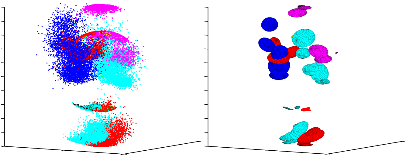 |
| A visualization of the conditional distributions for each part. (left) individual samples for each part; (right) fitting a covariance to the samples generated from each covariance. (Red - left foot, left knee and right elbow. Dark blue - right hand. Purple - left elbow and head. Light blue - right foot, right knee and right hand.) |
Observational Likelihoods
A part is represented by a rectangular patch with two image cues exploited, edges and color. Edge cues are extracted using a set of M overlapping HOG features placed along the edges of the part. Color is exploited by placing a bounding box at the location of the root node and then learning a foreground model using the pixel values within the box and a model for the background using pixels outside the box. The models are learnt using a GMM. This creates a very crude and noisy foreground probability map. The likelihood is then calculated as the average foreground probability value encompassed by the part. The individual likelihoods for each cue (edge, color) are then combined by product to produce the observational likelihoods.
Example results - samples generated by model representation and training data
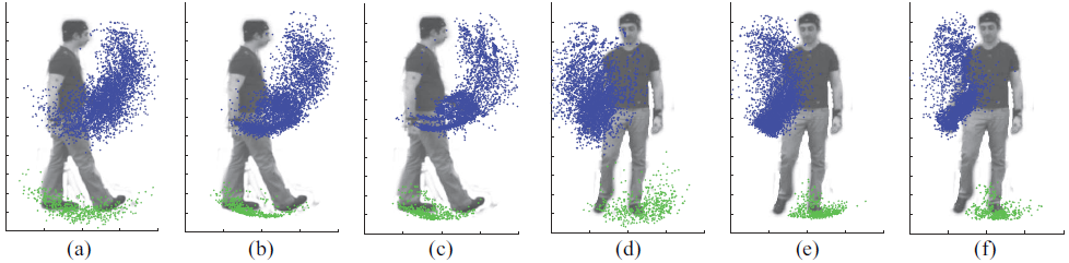 |
| Comparing samples of the left foot (green) and right wrist (blue) generated by each model representation and the training data. Side view: (a) loose limbed model (b) rigid joint model (c) training data; frontal view: (d) loose limbed model (e) rigid joint model (f) training data. |
Example results - model convergence after some iterations
| Loose Limbed Model | 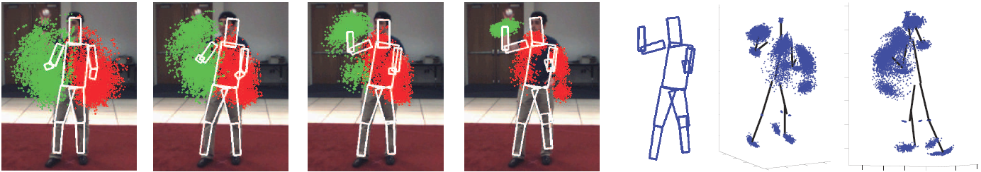 |
| Rigid Joint Model | 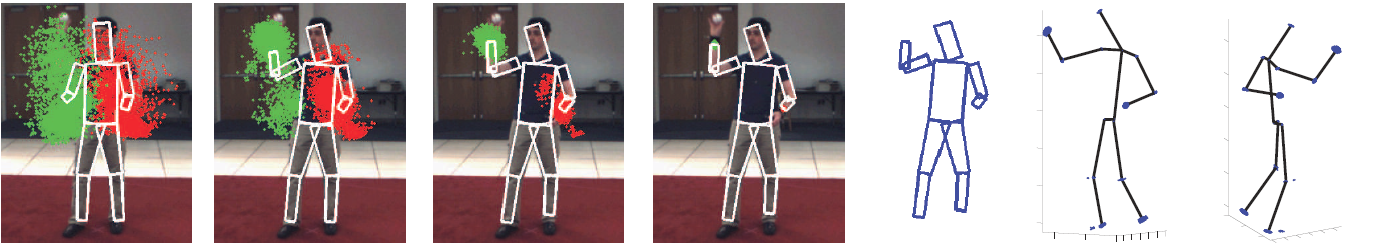 |
| Example of model convergence after (from left to right) 1, 3, 5, 10 iterations. Samples for the left (red) and right (green) wrist drawn from each prior are also shown as is the expected pose. The last three columns show the final expected pose, 3D reconstruction with samples that have been drawn from the final model, respectively. |
Example results - the expected pose after some iterations
 |
| Example frames showing the expected pose after (from left to right) 1, 3, 5, 7, and 10 iterations, projected onto the image (top) and in 3-D (bottom). The last figure at the bottom shows the final 3-D pose viewed from a different orientation. (The red and green samples show samples for the left and right wrists, respectively.) |
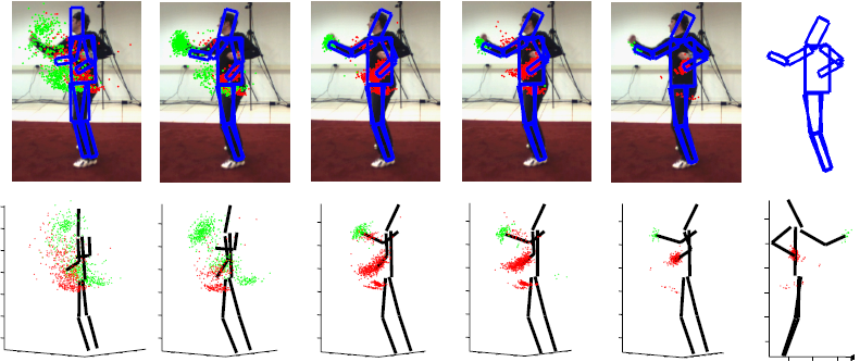
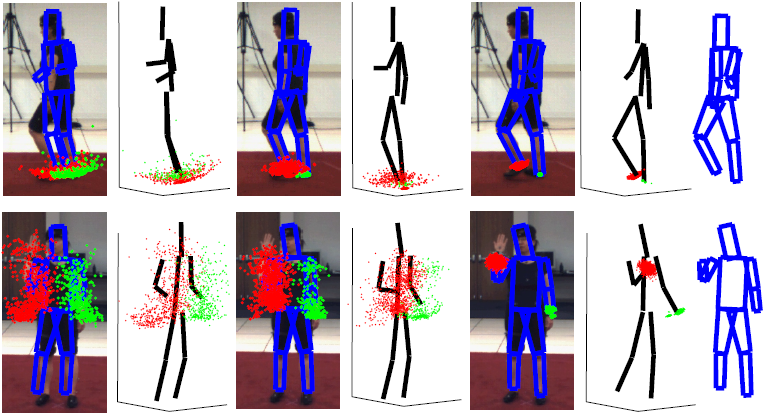 |
| Example frames showing the expected pose after (from left to right) 1, 4, and 10 iterations, projected onto the image and in 3-D. (The red samples show samples for the right foot (top) and right wrist (bottom); blue points depict the samples for the opposing parts.) |
Publications
- B. Daubney and X. Xie, Entropy Driven Hierarchical Search for 3D Human Pose Estimation, In Proceedings of the 22nd British Machine Vision Conference, September 2011.
- Ben Daubney and Xianghua Xie, Estimating 3D Human Pose from Single Images using Iterative Refinement of the Prior, In Proceedings of the 20th International Conference on Pattern Reconition, August 2010.
- Ben Daubney and Xianghua Xie, Estimating 3D Pose via Stochastic Search and Expectation Maximization, In Proceedings of the 6th Conference on Articulated Motion and Deformable Objects, July 2010.